Introduction
In its broadest sense, generative modeling addresses the statistical challenge of estimating and sampling from an unknown probability distribution given only a finite set of samples. When the target distribution is high-dimensional, this task becomes daunting, and traditional approaches such as Gaussian Mixture Models quickly become computationally infeasible [1]. Modern generative modeling techniques have largely circumvented these limitations by focusing on learning a mapping from a simple base distribution, which is easy to sample from, to the target distribution, approximating this mapping using the available data. The specifics of how this mapping is defined and constructed vary significantly across methods. Over the past decade, several approaches leveraging deep neural networks have emerged, including Variational Autoencoders (VAEs) [2], Generative Adversarial Networks (GANs) [3], Normalizing Flows [4], Denoising Diffusion Probabilistic Models (DDPMs) [5], and Score-Based Diffusion Models (SBMs) [6].
Among these frameworks, SBMs and DDPMs have achieved remarkable success across a wide range of applications, from image generation and protein design to weather forecasting, robotic manipulation, and climate emulation. SBMs model the mapping from the base to the target distribution as the reverse stochastic differential equation (SDE) of a pre-defined forward Ornstein-Uhlenbeck (OU) process, while DDPMs can be seen as a discrete counterpart of SBMs. In these models, the forward process gradually transforms samples from the target distribution into the base distribution by adding Gaussian noise with specified covariance structures. The reverse process similarly involves adding Gaussian noise to samples from the base distribution, effectively producing samples that mimic the target distribution. However, due to the nature of the OU process, the added noise is inherently Gaussian.
While this Gaussian constraint works well in many scenarios, it can be limiting when the target distribution exhibits heavy-tailed (rare and extreme events) or long-tailed (imbalanced datasets) characteristics. Recent works argue that Gaussian noise, with its square-exponentially decaying tails, inherently biases the generation process toward frequent, central samples in the training data, often underrepresenting rare or extreme samples that are at least equally critical. This limitation in diversity poses challenges in domains where extreme events or class imbalances are naturally present, as observed in various scientific and engineering contexts (e.g., [8]).
To address this limitation, recent studies have explored replacing Gaussian noise and Brownian motions with heavy-tailed noise or stochastic processes [7, 12, 13, 14]. While these works report improvements using metrics such as the Fréchet Inception Distance (FID) and Inception Score, these metrics, widely used in image generation tasks, are not particularly suited to assessing whether generative models effectively capture the tails of a distribution. In our view, this represents a significant gap in the current literature.
Motivated by this gap, we propose an alternative evaluation framework grounded in mathematical rigor and physical intuition, aimed at better assessing the impact of heavy-tailed noise on capturing rare and extreme events. Our approach consists of four steps: (1) selecting a dataset that naturally exhibits heavy tails, such as precipitation data, (2) identifying a physical aggregate quantity that characterizes the heavy-tail phenomenon, such as order statistics, (3) comparing the probability density of this aggregate quantity for both the original dataset and the samples generated by the model, and (4) computing tail-emphasizing statistics, such as those developed in [9, 10], to quantify differences. In particular, we focus on a representative type of heavy-tailed diffusion models (HTDM), the Lévy-Itō Models, and compare its ability to reproduce the tail events with SBMs when they are both trained on precipitation data.
Since this blog prioritizes accessibility over formalism, we focus on intuition and provide sufficient mathematical background for clarity. Rather than claiming that our approach is state-of-the-art, we aim to demonstrate the value of designing evaluation strategies from first principles. We hope this exposition inspires readers to reconsider the ways in which generative models are evaluated, particularly in contexts involving rare and extreme events.
Problem Statement
Let $p_0$ denote the true data distribution from which we have access to independent and identically distributed (IID) samples $\{x_i\}_{i=1}^n$, where $x(0)$ represents the corresponding random variable. Similarly, let $p_T$ be a known and tractable distribution from which samples can be easily generated, and let $x(T)$ denote its corresponding random variable.
The goal of generative modeling is to learn a mapping $\tau$ such that the push-forward distribution of $p_T$ under $\tau$ matches $p_0$, expressed mathematically as: \[\tau_{\#} p_T = p_0\] where $\tau_{\#} p_T$ represents the push-forward of $p_T$ by $\tau$. Intuitively, this means that for a sample $\xi \sim p_T$, applying the map $\tau$ transforms it into a sample $\tau(\xi)$ that follows $p_0$.
Score-Based Diffusion Models
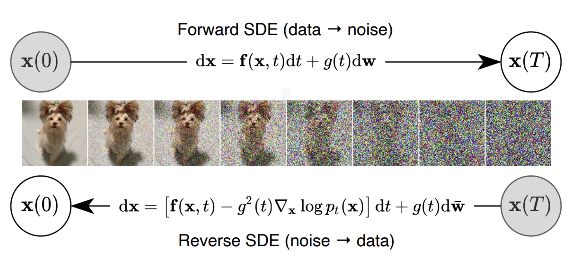
Score-based diffusion models (SBMs) define the mapping $\tau$ using an Ornstein-Uhlenbeck (OU) process, as illustrated in Figure 1.
 |
|---|
| Figure 1: Forward and backward processes of a diffusion model[6] |
SBMs consist of two key processes. In the forward process, each $x_i \sim p_0$ is progressively transformed into $\xi_i \sim p_T$ by adding Gaussian noise at each step. In the backward process, a sample $\xi \sim p_T$ is iteratively refined through a reverse process to produce $x \sim p_0$, effectively reconstructing the original data distribution.
It is important to note that Gaussian noise is applied during both the forward and backward processes. Figure 2 [homework] provides a visualization of the OU diffusion process, demonstrating the transformation of a bimodal Gaussian distribution into a unimodal Gaussian distribution in 1-D.
 |
|---|
| Figure 2: Visualization of the Ornstein-Uhlenbeck diffusion process [Homework 4] |
The Lévy-Itō Model
While SBMs have demonstrated outstanding performance across many applications, recent studies have highlighted their limitations in effectively covering the true distribution when the training dataset is imbalanced—for example, if 90% of the images are of dogs and only 10% are of cats. This limitation arises because Gaussian noise has light tails, causing sample trajectories to concentrate around frequent samples in the training data while neglecting under-represented samples. This imbalance often results in poor coverage of minority classes. Motivated by this drawback, recent works have proposed the use of heavy-tailed noise in the measure-transportation process.
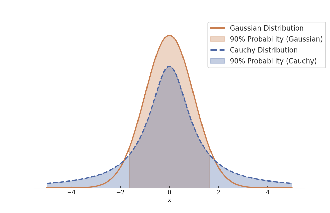
To intuitively understand the advantage of heavy-tailed noise over Gaussian noise, consider a comparison between a standard Gaussian distribution and a standard Cauchy distribution. Figure 3 illustrates the 90% centered probability coverage for each distribution. The range of values covered by the Cauchy distribution is more than twice that of the Gaussian, reflecting the heavier tail of the Cauchy distribution. This wider range implies that samples from the Cauchy distribution exhibit greater diversity compared to those from the Gaussian distribution. Incorporating such heavy-tailed noise into the diffusion process is the fundamental idea behind heavy-tailed diffusion models.
 |
|---|
| Figure 3: Gaussian vs Cauchy distribution |
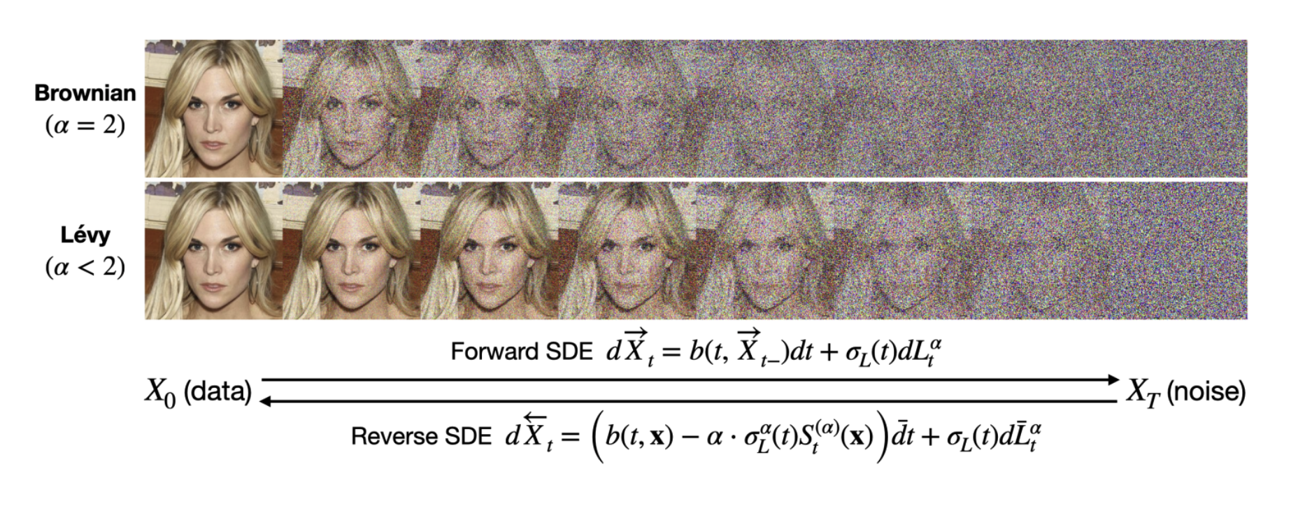
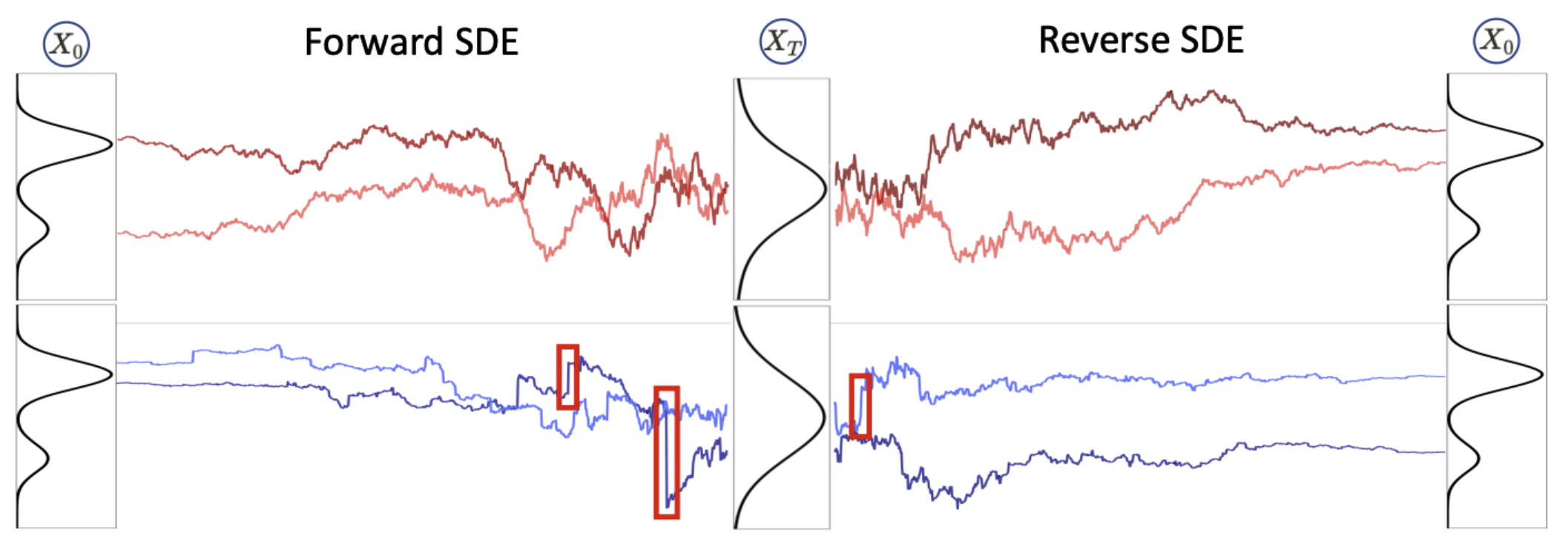
To explore this concept, we examine a representative model in this category: the Lévy-Itō Model (LIM). LIM replaces Gaussian noise with $\alpha$-stable noise, which has heavier tails. In the continuous case, the sample-transporting trajectories correspond to a Lévy process (when $\alpha < 2$) rather than a Brownian motion. Figure 4 provides an illustration of the LIM framework, and Figure 5 visualizes sample trajectories in a 1D-to-1D toy example.
 |
|---|
| Figure 4: Illustration of the Lévy-Itō Model [7] |
 |
|---|
| Figure 5: Visualization of sample trajectories in a 1D-to-1D toy example[7] |
Figure 4 presents the mathematical formulation of the forward and backward processes in the Lévy-Itō Model (LIM). The forward process in LIM is governed by the following stochastic differential equation:
\[ d X_t = b \left(t, X_{t-}\right) d t + \sigma_L(t) d L_t^\alpha, \]
where $b$ is the drift term, $\sigma_L$ is the variance schedule, and $L_t^\alpha$ represents an $\alpha$-stable Lévy process. Conversely, the backward process can be expressed as:
\[ d \overleftarrow{X}_t = \left(b(t, \mathbf{x}) - \alpha \cdot \sigma_L^\alpha(t) S_t^{(\alpha)}(\mathbf{x})\right) \bar{d} t + \sigma_L(t) d \bar{L}_t^\alpha,\]
where $S_t^{(\alpha)}$ is defined as:
\[S_t^{(\alpha)}(\mathbf{x}) := \frac{\Delta^{\frac{\alpha-2}{2}} \nabla p_t(\mathbf{x})}{p_t(\mathbf{x})},\]
and $\Delta^{\frac{\alpha-2}{2}}$ is the fractional Laplacian operator.
To avoid delving too deeply into mathematical intricacies, we summarize the core intuition behind these formulations. The differential of the $\alpha$-stable Lévy process introduces noise into the samples, analogous to the Gaussian noise in Score-Based Models (SBMs). When $\alpha = 2$, the process reduces to Brownian motion. However, for $\alpha < 2$, the process exhibits frequent, steep jumps characteristic of heavy-tailed noise, as highlighted in the red boxes of Figure 5.
The operator $S_t^{(\alpha)}$ serves a similar purpose to the score function in SBMs, enabling a closed-form expression for the backward process. While the fractional Laplacian operator is mathematically defined through the Fourier transform rather than conventional derivatives, its detailed properties are beyond the scope of this discussion.
In essence, both the forward and backward processes in LIM are similar to SBMs in terms of the formulations, with the critical difference being the inclusion of heavy-tailed noise.
Existing Evaluations
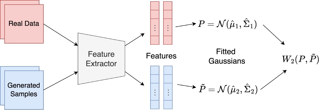
Many claims about the effectiveness of heavy-tailed diffusion models center on their purported ability to improve the coverage of the data distribution. However, to the best of our knowledge, these claims are predominantly supported by reductions in numerical scores from metrics such as the Fréchet Inception Distance (FID). Figure 6 provides an illustration of how FID is computed and used.
 |
|---|
| Figure 6: Illustration of the Fréchet Inception Distance |
At its core, FID quantifies the similarity between the real data distribution and the distribution of samples generated by a model. It achieves this as follows. Let $\{x_i\}^n_{i=1}$ represent the real data and $\{y_i\}^m_{i=1}$ the model-generated samples. Using a high-fidelity feature extractor $f$, such as the Inception v3 model pretrained on ImageNet [15, 16], the features of $x_i$ and $y_j$ are obtained as: \[f_i = f(x_i) \quad \text{and} \quad g_j = f(y_j), \quad \forall \, i, \, j.\] The empirical mean and covariance of the features for the real data are computed as: \[\mu_r = \frac{1}{n} \sum_{i=1}^n f_i, \quad \Sigma_r = \frac{1}{n} \sum_{i=1}^n (f_i - \mu_r)(f_i - \mu_r)^T.\] Similarly, the empirical mean and covariance of the features for the generated samples are: \[\mu_g = \frac{1}{m} \sum_{j=1}^{m} g_j, \quad \Sigma_g = \frac{1}{m} \sum_{j=1}^{m} (g_j - \mu_g)(g_j - \mu_g)^T.\] The FID is then defined as the 2-Wasserstein distance between the two Gaussian distributions $\mathcal{N}(\mu_r, \Sigma_r)$ and $\mathcal{N}(\mu_g, \Sigma_g)$, given by: \[\text{FID} = |\mu_r - \mu_g|_2^2 + \text{Tr}(\Sigma_r + \Sigma_g - 2(\Sigma_r \Sigma_g)^{1/2}),\] where $|\cdot|_2$ denotes the Euclidean norm, $\text{Tr}$ is the trace operator, and $(\Sigma_r \Sigma_g)^{1/2}$ represents the matrix square root of the product $\Sigma_r \Sigma_g$.
While FID has become the standard evaluation metric for image generation tasks, we argue that it falls short in assessing whether heavy-tailed diffusion models truly extend their coverage into the tail regions of the data distribution, due to the following limitations.
-
Focus on Central Tendency: FID primarily measures the alignment of the central moments (mean and covariance) of the distributions. It is not sensitive to rare samples or the behavior of the tails of the distributions.
-
Gaussian Assumption: By fitting Gaussians to the features, FID inherently disregards any non-Gaussian characteristics, which are critical when evaluating models designed to capture heavy tails.
-
Feature Extractor Bias: The choice of the feature extractor $f$ can heavily influence FID scores. If $f$ is not sensitive to tail samples, FID cannot adequately measure coverage in the tails.
-
Aggregate Nature: FID provides a single numerical score that does not distinguish between improvements in common regions of the distribution and improvements in rare or extreme regions.
Given these limitations, we believe that more targeted evaluation strategies are necessary to assess the ability of heavy-tailed diffusion models to capture rare and extreme events in the data distribution. In the next section, we propose a new evaluation framework designed to address these shortcomings.
A Physically Interpretable Evaluation Strategy
The limitations of existing evaluations are twofold: not only is the Fréchet Inception Distance (FID) insensitive to the tails of distributions, but also the image datasets commonly used in cited works are not naturally heavy-tailed. This is because most image datasets are curated to contain balanced and diverse samples across categories, ensuring uniform representation of common and rare events. Consequently, such datasets lack the inherent extreme-value behavior or power-law characteristics associated with heavy-tailed phenomena.
To address this, we propose testing models on datasets that are naturally heavy-tailed. With this motivation, we introduce the Physically Interpretable Tail Evaluation (PITE) strategy. This approach involves datasets representing physical phenomena that prior scientific research has demonstrated to follow heavy-tailed laws. Examples of such phenomena include precipitation levels, maximum sea levels, financial returns, genetic processes, network traffic, and Lagrangian trajectories [8]. Importantly, heavy-tailed phenomena are always defined with respect to specific physical properties, often referred to as physical observables or aggregate information, which are scalar quantities used to quantify the tails. These observables are known a priori based on domain knowledge.
The advantage of using naturally heavy-tailed datasets is clear: they provide an inherent notion of tails and a well-defined physical interpretation of the generated samples, allowing for meaningful evaluation of a model’s ability to capture rare or extreme events.
Once a well-defined notion of the tail is established, the challenge becomes quantifying the discrepancy between the tails of the real and generated distributions. Standard probabilistic metrics often fail in this regard because they emphasize the bulk of the distribution rather than the tails. For example, consider the Kullback-Leibler (KL) divergence between two distributions $p$ and $q$, defined as:
\[D_{KL}(p,q) = \int p(x)\log \frac{p(x)}{q(x)} dx.\]
Here, the log-density ratio is weighted by the density function $p(x)$. In tail regions, where $p(x)$ is small by definition, the contribution to the overall metric is negligible, making KL divergence insensitive to discrepancies in the tails.
To overcome this limitation, we adopt two tail-aware metrics from the rare-event quantification community: the Root Mean Squared Quantile Error (RMSQE) [10] and the Log Absolute Density Ratio (LOADER) metric [9].
-
Root Mean Squared Quantile Error (RMSQE):
The RMSQE metric focuses entirely on tail behavior. For two one-dimensional distributions $p$ and $q$, and a probability threshold $\eta$ (e.g., 0.95 or 0.99), it is defined as: \[\text{RMSQE}(p, q) := \int_\eta^1 \left|F_{p}^{-1}(u)-F_{q}^{-1}(u)\right|^2 du,\] where $F^{-1}$ denotes the pseudo-inverse of the cumulative distribution function (CDF) of the respective distribution. By integrating over extreme quantiles, RMSQE directly quantifies discrepancies in the tail regions. -
Log Absolute Density Ratio (LOADER):
The LOADER metric measures the divergence between two distributions with an emphasis on tail regions. It is defined as: \[\text{LOADER}(p,q) := \int \left|\log \frac{p(x)}{q(x)}\right|dx.\] While LOADER considers the entire distribution, it has been mathematically proven to emphasize tail behavior [9].
Practical Approximations
In practice, the metrics above are computed as follows.
- RMSQE: This metric is approximated using empirical quantiles from the data and model-generated samples.
- LOADER: The densities $p(x)$ and $q(x)$ are estimated using Kernel Density Estimation (KDE), and the integral is computed via efficient quadrature rules.
Summary of the PITE Strategy
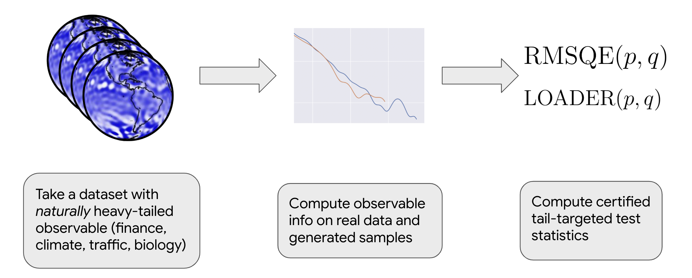
The PITE strategy involves the following steps, as visualized in Figure 7:
- Select a dataset that is naturally heavy-tailed.
- Compute the physically meaningful observable statistics (e.g., precipitation extremes, maximum returns).
- Evaluate the rare-event test statistic using tail-aware metrics such as RMSQE or LOADER.
By focusing on datasets with inherent tail behavior and using metrics designed to quantify discrepancies in the tails, the PITE strategy provides a rigorous and interpretable framework for evaluating generative models in contexts where rare and extreme events are critical.
 |
|---|
| Figure 7: Illustration of Our Physically Interpretable Tail Evaluation strategy |
Results
This section provides an overview of the experimental setup, along with quantitative and qualitative results.
Dataset
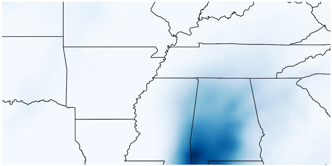
We use the ERA5-Land precipitation dataset, focusing on a region defined by latitudes $30.8^\circ$N to $38.7^\circ$N and longitudes $81.7^\circ$W to $97.6^\circ$W. The dataset has a spatial resolution of $0.1^\circ$ in each dimension, resulting in snapshots of size $80 \times 160$. Over 25 years, we collect daily maximal precipitation fields, yielding a total of 9050 snapshots. The physical observable used is the maximal regional daily maximum precipitation. Mathematically, if the dataset is represented as $\{x_i\}_{i=1}^{9050}$, the observable information is $\{\max x_i\}_{i=1}^{9050}$. A sample snapshot from the dataset is shown in Figure 8.
 |
|---|
| Figure 8: A sample snapshot from the ERA5-Land precipitation dataset |
Training and Generation
We train a Score-Based Model (SBM) and a Lévy-Itō Model (LIM) on the dataset, with hyperparameters tuned for optimal performance. For the LIM, we select $\alpha = 1.7$ to ensure the noise exhibits heavy-tailed behavior. Both models use a U-Net architecture. After training, each model generates 9050 sample snapshots to match the size of the training set, ensuring a fair comparison. The generated samples are denoted as $\{s_i\}_{i=1}^{9050}$ for SBM and $\{l_i\}_{i=1}^{9050}$ for LIM.
RMSQE and LOADER Values
After generating samples, we compute the observable information $\{\max s_i\}_{i=1}^{9050}$ and $\{\max l_i\}_{i=1}^{9050}$ for SBM and LIM, respectively. For the RMSQE metric, we set the tail cutoff $\eta = 0.975$, focusing on the top $2.5\%$ of quantiles. RMSQE is calculated between $\{\max x_i\}_{i=1}^{9050}$ and $\{\max s_i\}_{i=1}^{9050}$, and between $\{\max x_i\}_{i=1}^{9050}$ and $\{\max l_i\}_{i=1}^{9050}$.
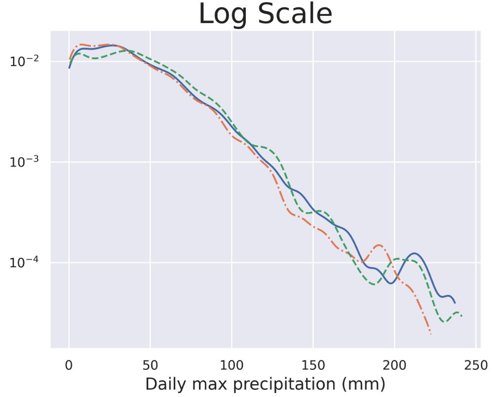
To compute LOADER, we first estimate the densities of $\{\max x_i\}_{i=1}^{9050}$, $\{\max s_i\}_{i=1}^{9050}$, and $\{max l_i\}_{i=1}^{9050}$ using Kernel Density Estimation (KDE) accelerated with Fast Fourier Transform (FFT). The resulting densities are denoted as $p_x$, $p_s$, and $p_l$. LOADER values are then calculated using Gaussian quadrature rules for $\text{LOADER}(p_x, p_s)$ and $\text{LOADER}(p_x, p_l)$. The estimated densities are shown in Figure 9, where the blue curve represents $p_x$, the orange curve represents $p_s$, and the green curve represents $p_l$.
 |
|---|
| Figure 9: Comparison of approximate densities of the physical observable information associated with the original dataset, samples generated by SBM, and samples generated by LIM. Blue: original. Orange: SBM. Green: LIM. |
The quantitative results are summarized below:
| Metric | SBM | LIM ($\alpha = 1.7$) |
|---|---|---|
| RMSQE | 47.68 | 12.74 |
| LOADER | 57.83 | 38.27 |
Analysis of Results
The results clearly demonstrate that LIM outperforms SBM in both RMSQE and LOADER metrics. This is also evident in Figure 9, where the tail of $p_l$ closely aligns with $p_x$, whereas $p_s$ diverges significantly. It is worth noting that LIM’s improvement in the RMSQE metric is much more pronounced than in the LOADER metric. This difference arises because RMSQE exclusively focuses on tail behavior, while LOADER accounts for the entire distribution, including the bulk. In the bulk regions, SBM slightly outperforms LIM due to LIM’s emphasis on tail generation, which comes at the expense of bulk accuracy. This trade-off is consistent with the intended purpose of heavy-tailed noise.
In summary, this example and the corresponding tail-aware metrics illustrate that employing heavy-tailed noise, as in LIM, can significantly enhance a model’s ability to generate tail events effectively.
Conclusion
We have proposed an alternative evaluation strategy for assessing the ability of heavy-tailed diffusion models to capture under-represented regions of the data distribution. Our framework, named Physically Interpretable Tail Evaluation (PITE), is grounded in well-established physical principles and offers a quantitative approach to evaluate generative models in terms of their capacity to generate tail events. By focusing on datasets with naturally heavy-tailed properties and employing tail-aware metrics such as RMSQE and LOADER, PITE provides a more rigorous and interpretable assessment compared to traditional metrics like Fréchet Inception Distance (FID).
Our findings corroborate claims made in recent works on heavy-tailed diffusion models, showing that replacing Gaussian noise with heavy-tailed noise improves the model’s ability to generate samples from the tail regions of the data distribution. Specifically, the Lévy-Itō Model (LIM), with $\alpha$-stable noise, demonstrated significantly better performance than standard Score-Based Models (SBMs) in generating tail events. This improvement was reflected in lower RMSQE and LOADER values and was further supported by visual alignment of the generated tail densities with the true data distribution.
The PITE framework goes beyond merely improving evaluation accuracy; it offers a physically interpretable lens through which model performance can be understood in the context of rare and extreme events. This is particularly relevant for applications such as weather forecasting, financial risk analysis, and scientific simulations, where accurate modeling of tails is crucial.
References
[1] Bishop, Christopher M., and Nasser M. Nasrabadi. Pattern recognition and machine learning. Vol. 4. No. 4. New York: springer, 2006.
[2] Kingma, Diederik P., and Max Welling. “Auto-Encoding Variational Bayes.” 2nd International Conference on Learning Representations (ICLR), 2014.
[3] Goodfellow, Ian, et al. “Generative adversarial nets.” Advances in neural information processing systems 27 (2014).
[4] Rezende, Danilo, and Shakir Mohamed. “Variational inference with normalizing flows.” International conference on machine learning. PMLR, 2015.
[5] Ho, Jonathan, Ajay Jain, and Pieter Abbeel. “Denoising diffusion probabilistic models.” Advances in neural information processing systems 33 (2020): 6840-6851.
[6] Song, Yang, et al. “Score-based generative modeling through stochastic differential equations.” arXiv preprint arXiv:2011.13456 (2020).
[7] Yoon, Eun Bi, et al. “Score-based generative models with Lévy processes.” Advances in Neural Information Processing Systems 36 (2023): 40694-40707.
[8] Coles, Stuart, et al. An introduction to statistical modeling of extreme values. Vol. 208. London: Springer, 2001.
[9] Mohamad, Mustafa A., and Themistoklis P. Sapsis. “Sequential sampling strategy for extreme event statistics in nonlinear dynamical systems.” Proceedings of the National Academy of Sciences 115.44 (2018): 11138-11143.
[10] Blanchard, Antoine, et al. “A multi-scale deep learning framework for projecting weather extremes.” arXiv preprint arXiv:2210.12137 (2022).
[11] Heusel, Martin, et al. “Gans trained by a two time-scale update rule converge to a local nash equilibrium.” Advances in neural information processing systems 30 (2017).
[12] Kushagra Pandey, Jaideep Pathak, Yilun Xu, Stephan Mandt, Michael Pritchard, Arash Vahdat, and Morteza Mardani. Heavy-Tailed Diffusion Models, October 2024. arXiv:2410.14171.
[13] Dario Shariatian, Umut Simsekli, and Alain Durmus. Denoising Lévy Probabilistic Models, July 2024. arXiv:2407.18609 [cs, stat].
[14] Eliya Nachmani, Robin San Roman, and Lior Wolf. Denoising Diffusion Gamma Models, October 2021. arXiv:2110.05948 [cs, eess].
[15] Szegedy, Christian, et al. “Rethinking the inception architecture for computer vision.” Proceedings of the IEEE conference on computer vision and pattern recognition. 2016.
[16] Deng, Jia, et al. “Imagenet: A large-scale hierarchical image database.” 2009 IEEE conference on computer vision and pattern recognition. Ieee, 2009.